UTU SEP Products: Very high-energy solar proton event database
Solar proton event database
This product provides a database of solar proton events observed above 300 MeV during solar cycles 22-24, i.e., between September 1986 and December 2019. In total, the database includes 68 events: 33 ground level events (GLEs 40-72), which have been detected with neutron monitors (NMs), and 35 events (referred to as solar proton events, SPEs) which have been detected with space-borne detectors above 300 MeV, but have not produced sufficient fluxes at high energies to be detected with ground level NMs.
The database includes differential fluence (time-integrated flux) and peak flux spectra in ten energies between 200 MeV and 7690 MeV for all of the events. In addition, flux spectra at 5-minute resolution around the high-energy peak of the event are provided for six of the well-observed GLEs (namely, GLEs 59, 60, 67, 70, 71 and 72). The full event list is given below.
| Event date | GLE | Note |
|---|---|---|
| 1989-05-20 | ||
| 1989-07-25 | 40 | |
| 1989-08-12 | ||
| 1989-08-16 | 41 | |
| 1989-09-29 | 42 | |
| 1989-10-19 | 43 | |
| 1989-10-22 | 44 | |
| 1989-10-24 | 45 | |
| 1989-10-29 | ||
| 1989-11-15 | 46 | |
| 1989-11-30 | ||
| 1990-05-21 | 47 | |
| 1990-05-24 | 48 | |
| 1990-05-26 | 49 | |
| 1990-05-28 | 50 | |
| 1991-03-23 | ||
| 1991-05-13 |
| Event date | GLE | Note |
|---|---|---|
| 1991-06-04 | ||
| 1991-06-11 | 51 | |
| 1991-06-15 | 52 | |
| 1991-10-30 | ||
| 1992-03-07 | ||
| 1992-06-25 | 53 | |
| 1992-11-02 | 54 | |
| 1997-11-04 | ||
| 1997-11-06 | 55 | |
| 1998-05-02 | 56 | |
| 1998-05-06 | 57 | |
| 1998-08-24 | 58 | |
| 1998-09-30 | ||
| 1998-11-14 | ||
| 2000-07-14 | 59 | * |
| 2000-11-08 | ||
| 2001-04-02 |
| Event date | GLE | Note |
|---|---|---|
| 2001-04-12 | ||
| 2001-04-15 | 60 | * |
| 2001-04-18 | 61 | |
| 2001-08-16 | ||
| 2001-09-24 | ||
| 2001-10-22 | ||
| 2001-11-04 | 62 | |
| 2001-11-22 | ||
| 2001-12-26 | 63 | |
| 2002-04-21 | ||
| 2002-08-24 | 64 | |
| 2003-10-28 | 65 | |
| 2003-10-29 | 66 | |
| 2003-11-02 | 67 | * |
| 2004-11-01 | ||
| 2004-11-10 | ||
| 2005-01-17 | 68 |
| Event date | GLE | Note |
|---|---|---|
| 2005-01-20 | 69 | |
| 2005-06-16 | ||
| 2005-09-08 | ||
| 2006-12-06 | ||
| 2006-12-13 | 70 | * |
| 2012-01-23 | ||
| 2012-01-27 | ||
| 2012-03-07 | ||
| 2012-03-13 | ||
| 2012-05-17 | 71 | * |
| 2013-05-22 | ||
| 2014-01-06 | ||
| 2014-01-07 | ||
| 2014-02-25 | ||
| 2014-09-01 | ||
| 2015-10-29 | ||
| 2017-09-10 | 72 | * |
Note '*' = 5-min spectra available
The fluence spectra are based on analyses of space-borne (GOES EPS + HEPAD) and NM observations, in which integral proton fluences were fitted with a Band function (BF; Tylka and Dietrich, 2009; Atwell et al., 2016; Raukunen et al., 2018). The Band function (Band et al., 1993) is a double power law function with four parameters: two spectral indices γ1 and γ2, roll-over rigidity R0 and fluence normalization factor J0. More recently, the GLE spectra were revised by Koldobskiy et al. (2021) using an updated NM yield function. The revised spectra were fitted with a modified Band function (MBF), which differs from the Band function by an additional exponential roll-over at high rigidities. Thus, the MBF has five fitted parameters: two spectral indices γ1 and γ2, roll-over rigidities R1 and R2 and a high-rigidity fluence normalization factor J2.
In the database, the fluence spectra of GLEs have been calculated by numerically differentiating the MBF representations, with the exception of GLEs 51, 54, 57 and 68, for which the BF representations were used. The spectra of all SPEs have been calculated by numerically differentiating the BF representations. The parameters of all spectral representations can be found in Vainio et al. (2017), Raukunen et al. (2018) and Koldobskiy et al. (2021).
As the available space-borne observations reach only ~600 MeV (Raukunen et al., 2020), and detailed, time-resolved fluxes from NM observations are available for only a few events, extrapolation is required to calculate the peak flux spectra. In the database we calculate the peak flux spectra by scaling the fluence spectra. More precisely, we first calculate the integral peak fluxes I(>E) for all events at >100 MeV and >400 MeV using the >100 MeV GOES/EPS channel and integral bow-tie analysed GOES/HEPAD channels P9 and P10. Then we select events where the >400 MeV peak flux is greater than two times the background flux, and compare the ratios RI = I(>100) / I(>400) with the corresponding fluence ratios, i.e., RF = F(>100) / F(>400). We find that, on average, RF = 1.591 · RI, meaning that the peak flux spectra are harder with a difference of log(1.591) / log(4) = 0.335 in spectral index. The scaling coefficient is calculated as c = I(>E0) / F(>E0), where E0 = 400 MeV if the background condition is fulfilled and E0 = 100 MeV otherwise. Thus, we calculate the scaled and corrected integral peak flux spectra as Icorr(>E) = c · F(>E) · (E/E0)0.335.
The flux spectra for the selected, well-observed GLEs are based on the inversion method described in Mishev et al. (2014). The method depends on detailed modeling of the particle transport in the geomagnetic field and the Earth’s atmosphere as well as the detection efficiency of NMs to determine the spectral and angular characteristics of solar energetic particles (SEPs) near Earth.
User instructions
Proton event spectrum tool
This tool lets the user plot and download the spectrum of a selected data type and event. First, the user selects the data type (either Fluence, Peak flux or Flux). That selection determines the list of events available for plotting: for Fluence and Peak flux, the full list of >300 MeV proton events observed during solar cycles 22-24 is available. For flux, the event list narrows down to six well-observed GLEs, and after selecting an event, an additional selection of a time interval becomes available.
When selecting, for example, peak flux spectrum for GLE 72, the result should look like this:
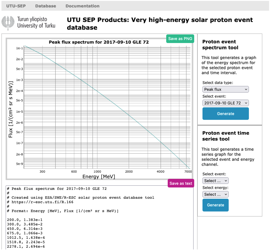
The user can hover over the plot area and read the values of the points closest to the cursor on the screen. The plot, once created, can also be saved as a PNG file using the button on the right. Alternatively, the raw data of the plot in numeric format can be copied and pasted out from the text field below the plot area, or downloaded as a text file using the "Save as text"-button.
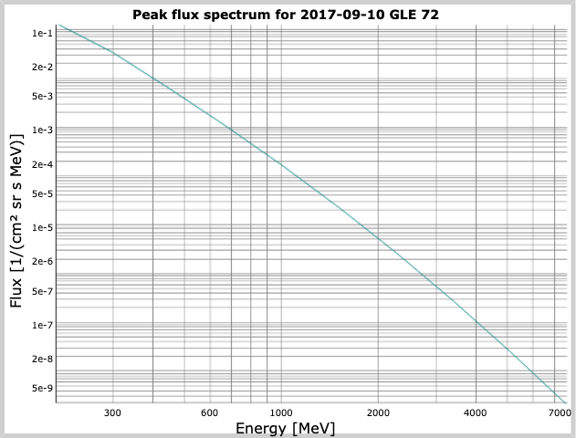
In case the user clicks the green button to save the PNG file, either a file download dialog appears or the plot is downloaded automatically into the default download folder, depending on the browser settings. The saved plot should look like this:
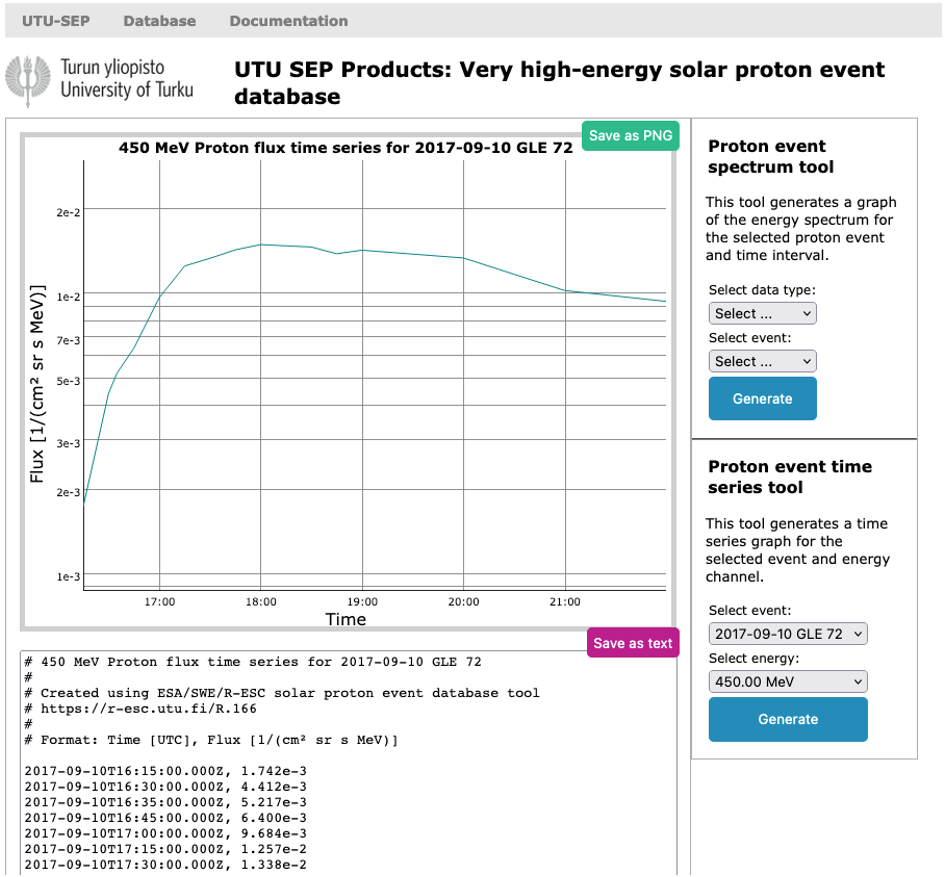
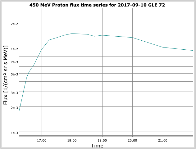
Proton event time series tool
This tool lets the user plot and download the differential flux time series at a selected energy for a selected event. For example, selecting the flux time series for GLE 72 at 450 MeV should produce results like this:
Machine-to-machine interfaces
The machine-to-machine interface (API) to the product is provided as a web page located at
https://r-esc.utu.fi/api/R.166/<tool>?<parameter_list>
Here <tool> is either the string ‘spectrum’ or the string ‘timeseries’ for accessing the spectrum tool or the time series tool, respectively. The <parameter_list> depends on the chosen tool, as explained below.
The spectrum tool has two parameters:
| Parameter name | Type | Range / allowed values | Description |
|---|---|---|---|
| type | string | "fluence" or "peakflux" | Data type selector between fluence or peak flux |
| event | string |
"1989-05-20",
"1989-07-25", "1989-08-12", "1989-08-16", "1989-09-29", "1989-10-19", "1989-10-22", "1989-10-24", "1989-10-29", "1989-11-15", "1989-11-30", "1990-05-21", "1990-05-24", "1990-05-26", "1990-05-28", "1991-03-23", "1991-05-13", "1991-06-04", "1991-06-11", "1991-06-15", "1991-10-30", "1992-03-07", "1992-06-25", "1992-11-02", "1997-11-04", "1997-11-06", "1998-05-02", "1998-05-06", "1998-08-24", "1998-09-30", "1998-11-14", "2000-07-14", "2000-11-08", "2001-04-02", "2001-04-12", "2001-04-15", "2001-04-18", "2001-08-16", "2001-09-24", "2001-10-22", "2001-11-04", "2001-11-22", "2001-12-26", "2002-04-21", "2002-08-24", "2003-10-28", "2003-10-29", "2003-11-02", "2004-11-01", "2004-11-10", "2005-01-17", "2005-01-20", "2005-06-16", "2005-09-08", "2006-12-06", "2006-12-13", "2012-01-23", "2012-01-27", "2012-03-07", "2012-03-13", "2012-05-17", "2013-05-22", "2014-01-06", "2014-01-07", "2014-02-25", "2014-09-01", "2015-10-29" or "2017-09-10" |
Event selector |
The list of events available in the spectrum tool can also be acquired by accessing the following web page:
https://r-esc.utu.fi/api/R.166/spectrum/eventlist
The output of the API spectrum tool for an event is identical to the GUI except for the header part, which is omitted.
For example, acquiring the peak flux spectrum of GLE 72 on September 10, 2017, access the following web page:
https://r-esc.utu.fi/api/R.166/spectrum?type=peakflux&event=2017-09-10
The time series tool has one mandatory and one optional parameter:
| Parameter name | Type | Range / allowed values | Description |
|---|---|---|---|
| event | string |
"2000-07-14",
"2001-04-15", "2003-11-02", "2006-12-13", "2012-05-17" or "2017-09-10" |
Event selector (mandatory) |
| energy_channel | integer | 1 — 10 | Energy channel (optional) (see below for corresponding MeV values) |
energy_channel value index correspondence to energy value:
| energy_channel | Description |
|---|---|
| 1 | 200 MeV |
| 2 | 300 MeV |
| 3 | 450 MeV |
| 4 | 675 MeV |
| 5 | 1012.5 MeV |
| 6 | 1518.8 MeV |
| 7 | 2278.1 MeV |
| 8 | 3417.2 MeV |
| 9 | 5125.8 MeV |
| 10 | 7688.7 MeV |
If the energy channel parameter is omitted, the tool returns the time series for all 10 channels; in this case, the output has 11 columns: column 1 gives the time stamp and columns 2-11 give the flux time series for energy channels 1-10.
The list of events available in the time series tool can also be acquired by accessing the following web page:
https://r-esc.utu.fi/api/R.166/timeseries/eventlist
The output of the API time series tool for an event and an energy channel is identical to the GUI except for the header part, which is omitted.
For example, acquiring the 200 MeV flux time series of GLE 72 on September 10, 2017, access the following web page:
https://r-esc.utu.fi/api/R.166/timeseries?event=2017-09-10&energy_channel=1
References
Atwell W. et al., 2016, In Proc. 46th International Conference on Environmental SystemsBand D. et al., 1993, Astrophysical Journal, 413, 281, DOI: 10.1086/172995
Koldobskiy S. et al., 2021, Astronomy & Astrophysics, 647, A132, DOI: 10.1051/0004-6361/202040058
Mishev, A. et al., 2014, Journal of Geophysical Research: Space Physics, 119, 2, DOI: 10.1002/2013JA019253
Raukunen, O. et al., 2018, Journal of Space Weather and Space Climate, 8, A04, DOI: 10.1051/swsc/2017031
Raukunen, O. et al., 2020, Journal of Space Weather and Space Climate, 10, 24, DOI: 10.1051/swsc/2020024
Tylka A.J. and Dietrich W.F., 2009, In Proc. 31st International Cosmic Ray Conference
Vainio R. et al., 2017, Astronomy & Astrophysics, 604, A47, DOI: 10.1051/0004-6361/201730547